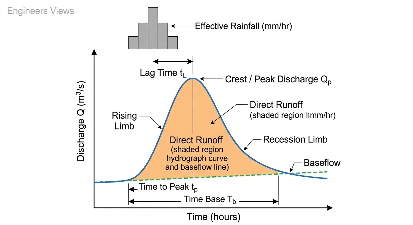
Figure 1: Annotated flood hydrograph showing all key components and time parameters.
Introduction to Hydrographs
A hydrograph is a graphical representation of the variation of discharge (or stage) of a stream at a given gauging station plotted against time. In hydrology, it is the single most important tool for understanding and quantifying the rainfall-runoff response of a catchment. Every flood estimate, reservoir design, culvert sizing, and floodplain mapping exercise depends either directly on a measured hydrograph or on a model capable of reproducing one.
The term was popularized in the early twentieth century when engineers began systematically recording river levels and flows. Today, digital sensors transmit real-time flow data globally, but the fundamental shape and the physics it encodes remain exactly as described by the pioneers of engineering hydrology.
Key definition: A hydrograph expresses the integrated response of an entire catchment to a rainfall event, capturing the combined effects of precipitation intensity, basin geometry, soils, land use, antecedent moisture, and channel hydraulics.
Components of a Flood Hydrograph
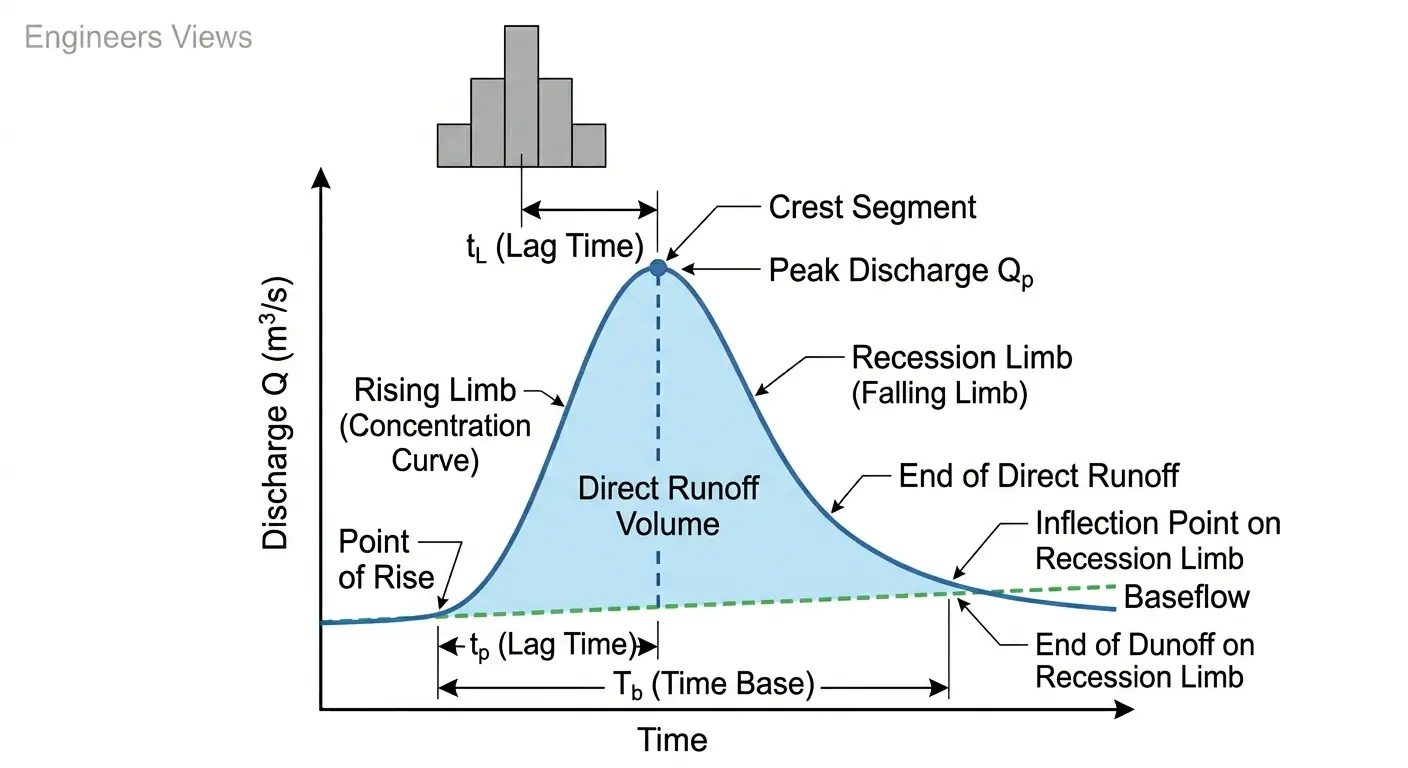
Figure 2: Labelled components of a single-storm flood hydrograph.
Rising Limb (Concentration Curve)
The rising limb extends from the point of initial rise in streamflow to the point of peak discharge. Its shape reflects the increasing contribution of runoff from successive parts of the catchment as rainfall continues. Steep rising limbs indicate fast-responding, impervious, or small basins; gentle slopes indicate large, permeable, or heavily forested catchments.
Crest Segment
The crest segment includes the peak discharge $Q_p$ and a short interval on either side where the hydrograph is relatively flat. The time to peak $t_p$ is measured from the centroid of effective rainfall to $Q_p$. Some references measure $t_p$ from the start of rainfall or from the start of runoff.
Recession Limb (Falling Limb)
The recession limb begins at the peak and extends to the point where direct runoff ceases. It represents the withdrawal of water from storage in the channel and overland flow zones. Barnes (1940) showed that the recession follows an exponential decay:
where $Q_t$ is discharge at time $t$ after the start of the recession interval, $Q_0$ is the discharge at that starting point, and $K_r$ is the recession constant (units: time$^{-1}$). The equation is equivalently written in the power form:
where $K$ is a dimensionless recession constant ($0 < K < 1$), typically 0.90 to 0.99 for large basins on a daily time step.
Time Parameters
| Parameter | Symbol | Definition |
|---|---|---|
| Lag time | $t_L$ | Time from centroid of effective rainfall to peak discharge |
| Time to peak | $t_p$ | Time from start of effective rainfall to peak discharge |
| Time of concentration | $t_c$ | Time for runoff to travel from the hydraulically most remote point to the outlet |
| Time base | $T_b$ | Total duration of direct runoff from start to end |
| Recession time | $T_r$ | Duration of recession limb from peak to end of direct runoff |
Baseflow
Baseflow (groundwater contribution) is the sustained low-flow component present before, during, and after the storm event. It must be separated from the hydrograph before unit hydrograph analysis can proceed. Three common separation methods are:
- Straight-line method: Draw a horizontal line from the point of rise to where it intersects the recession limb.
- Fixed base method: Extend the pre-event recession curve under the hydrograph, then connect it to the recession limb at a point $N$ days after the peak, where $N = A^{0.2}$ ($A$ in km²).
- Variable slope method: Project the pre-event recession forward and the post-event recession backward; join the two inflection points with a curved line.
Types of Hydrographs
Storm (Flood) Hydrograph
The hydrograph produced by a single storm event. It includes both direct runoff and baseflow. This is the raw record obtained from stream-gauging stations.
Annual Hydrograph
A plot of mean daily or monthly discharge over a full year, revealing the seasonal pattern of flow regime including wet-season peaks and dry-season low flows. Used in reservoir yield analysis and irrigation planning.
Composite Hydrograph
Results when multiple storm bursts occur in quick succession so that individual hydrographs overlap. Analysis requires separation of the individual storm responses.
Unit Hydrograph (UH)
The hydrograph of direct runoff resulting from one unit (1 mm or 1 cm) of effective rainfall uniformly distributed over the entire catchment at a uniform rate during a specified duration. This is the most important theoretical tool in deterministic hydrology, introduced by Sherman (1932).
Synthetic Unit Hydrograph
A unit hydrograph derived from catchment characteristics (area, slope, shape) rather than from observed rainfall-runoff data. Essential for ungauged catchments.
Instantaneous Unit Hydrograph (IUH)
The limiting case of a unit hydrograph as the rainfall duration approaches zero. It is a theoretical concept that provides the most fundamental description of basin response and forms the basis for convolution-based runoff modelling.
Factors Affecting the Shape of a Hydrograph
- Catchment area: Larger areas produce lower peak discharges per unit area and longer time bases.
- Basin shape: Fan-shaped (compact) basins produce sharp, high peaks; elongated basins produce flatter, delayed peaks.
- Slope: Steeper slopes lead to faster concentration and higher peaks.
- Drainage density: High drainage density reduces travel times, producing flashier hydrographs.
- Soil permeability and land use: Impervious surfaces increase runoff ratio and peak; forests and permeable soils attenuate peaks.
- Rainfall intensity and duration: Higher intensity over longer duration produces greater peak discharge.
- Antecedent moisture condition (AMC): Wet soils have lower infiltration capacity, increasing the runoff fraction.
- Channel storage: Lakes and floodplains attenuate peaks by storing flood water temporarily.
Unit Hydrograph Theory
Sherman's Assumptions (1932)
The classical unit hydrograph rests on three fundamental assumptions:
- Time invariance: The direct runoff hydrograph for a given effective rainfall pattern is always the same regardless of when the storm occurs. The basin's response function does not change with time.
- Linearity (superposition): The direct runoff from any effective rainfall pattern can be computed by multiplying the UH ordinates by the corresponding effective rainfall depths and superimposing the resulting hydrographs with appropriate time lags.
- Proportionality: If the effective rainfall in a given duration is $n$ units instead of 1, the direct runoff ordinates are $n$ times the UH ordinates.
Unit constraint: The volume under the unit hydrograph must equal exactly 1 unit (1 mm or 1 cm) of direct runoff over the entire catchment area. That is, $\sum Q_i \cdot \Delta t = A \times 1\,\text{mm} / 1000$ (with $Q$ in m³/s, $A$ in m², $\Delta t$ in seconds).
Superposition Principle
For a storm producing effective rainfall depths $P_1, P_2, \ldots, P_n$ in successive unit periods, the direct runoff hydrograph ordinate at time step $t$ is:
where $U_{t-(j-1)}$ is the unit hydrograph ordinate at time $[t-(j-1)]\Delta t$, and $P_j$ is the effective rainfall depth in the $j$-th time interval. This is the discrete convolution equation — the foundation of all linear rainfall-runoff models.
Changing the Duration of a Unit Hydrograph
A $t_r$-hour unit hydrograph can be converted to a $2t_r$-hour unit hydrograph by lagging two $t_r$-hour UHs by $t_r$ hours, adding their ordinates, and dividing by 2. More generally, the S-curve method (described below) is used to convert to any arbitrary duration.
Derivation of the Unit Hydrograph from Storm Data
To derive a UH from a gauged single-storm event, the following steps are followed:
-
Select a simple, isolated storm event with relatively uniform rainfall distribution over the catchment and a single peak in the hydrograph. Ideally use storms of moderate intensity with a near-uniform spatial pattern.
-
Separate baseflow from the total hydrograph using one of the three methods described above to obtain the direct runoff hydrograph (DRH).
-
Compute the direct runoff depth $P_e$ (effective rainfall) by dividing the volume of direct runoff $V_\text{DRH}$ by the catchment area $A$:$$P_e = \frac{V_\text{DRH}}{A} = \frac{\displaystyle\sum Q_i^\text{DRH} \cdot \Delta t}{A}$$
-
Divide each DRH ordinate by the effective rainfall depth $P_e$ to obtain the unit hydrograph ordinates:$$U_i = \frac{Q_i^\text{DRH}}{P_e}$$The resulting UH has a volume equivalent to exactly 1 unit of effective rainfall over the basin.
-
Determine the UH duration $t_r$: this is the duration of the effective rainfall burst used in the storm, not the total storm duration.
-
Average multiple UHs derived from several storms to reduce observational uncertainty. Ordinates may be averaged directly; time parameters should be aligned on the time axis before averaging.
Matrix (Least-Squares) Method for Complex Storms
For storms with multiple rainfall bursts, the convolution equation forms an overdetermined system of linear equations:
where $\mathbf{Q}$ is the vector of direct runoff ordinates, $\mathbf{P}$ is the lower-triangular matrix of effective rainfall depths, and $\mathbf{U}$ is the unknown UH ordinate vector. The least-squares solution is:
This approach is robust when data quality is good but can produce oscillating (physically unrealistic) solutions for noisy data, in which case constrained optimisation is applied.
S-Curve (Summation Curve) Method
The S-curve (also called the S-hydrograph) is used to convert a unit hydrograph of duration $t_r$ hours to any other duration $t_r'$ hours without restriction to simple multiples.
Construction of the S-Curve
The S-curve is produced by summing an infinite series of $t_r$-hour UHs, each lagged by $t_r$ hours from the previous one:
The resulting S-curve rises from zero to a constant equilibrium discharge $Q_\text{eq}$:
where $A$ is catchment area (m²) and $t_r$ is the unit duration in seconds. This equilibrium corresponds to a continuous rainfall of 1 mm/hr uniformly over the entire catchment.
Deriving a New UH from the S-Curve
- Lag the original S-curve by the desired new duration $t_r'$.
- Subtract the lagged S-curve from the original S-curve to get a stepped hydrograph.
- Multiply each ordinate by $t_r / t_r'$ to obtain the unit hydrograph for duration $t_r'$.
Oscillation warning: If the original UH contains data errors or irregular ordinates, the S-curve method can amplify these into unrealistic oscillations in the derived UH. Always smooth the original UH ordinates before applying the S-curve.
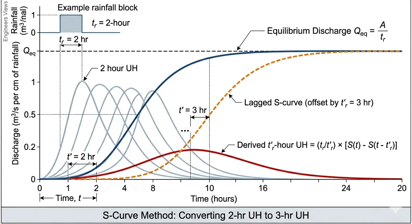
Figure 3: S-curve method for converting a 2-hour UH to a 3-hour UH.
Instantaneous Unit Hydrograph (IUH)
The IUH, denoted $u(t)$ or $h(t)$, is defined as the direct runoff hydrograph produced by an instantaneous burst of effective rainfall of 1 mm spread uniformly over the entire catchment. It is the limiting form of the unit hydrograph as duration $t_r \to 0$.
Nash Cascade Model
Nash (1957) modelled the IUH as the outflow from a cascade of $n$ identical linear reservoirs, each with storage constant $K$:
where $\Gamma(n)$ is the Gamma function, equal to $(n-1)!$ when $n$ is a positive integer. The two parameters $n$ and $K$ characterise the basin: $n$ controls the shape (skewness) and $K$ the scale (time). The moments of the IUH give:
Parameters $n$ and $K$ are estimated from the first two moments of the observed direct runoff hydrograph using the method of moments.
Relationship between IUH and Unit Hydrograph
The $t_r$-hour unit hydrograph ordinate $U(t,\, t_r)$ relates to the IUH by:
Conversely, the IUH is the derivative of the S-curve with respect to time:
Convolution Integral
For any effective rainfall intensity function $i(\tau)$, the direct runoff hydrograph is obtained by the convolution integral:
This is the continuous analogue of the discrete convolution used with the finite-duration UH. In practice it is evaluated numerically.
Synthetic Unit Hydrograph Methods
When observed rainfall-runoff data are not available (ungauged catchments), the UH is estimated from measurable basin characteristics. Three widely used methods are described below.
Snyder's Synthetic Unit Hydrograph
Snyder (1938) related UH parameters to basin characteristics for Appalachian watersheds:
where $t_p$ is the lag time (hours), $L$ is the main-channel length (km), $L_{ca}$ is the distance from the outlet to the point on the channel nearest the centroid of the basin (km), $A$ is basin area (km²), and $C_t$ (0.3 to 0.6) and $C_p$ (0.4 to 0.8) are regional empirical coefficients. Peak discharge $Q_p$ is in m³/s.
The standard UH duration for Snyder's method is:
SCS (NRCS) Dimensionless Unit Hydrograph
The U.S. Soil Conservation Service (now NRCS) developed a dimensionless UH expressed as $Q/Q_p$ versus $t/t_p$. The peak discharge is:
where $A$ is in km² and $t_p$ is in hours. The time to peak is estimated as:
where $t_c$ is the time of concentration. The time base of the SCS UH is approximately $T_b = 2.67\, t_p$.
| $t/t_p$ | $Q/Q_p$ | $t/t_p$ | $Q/Q_p$ |
|---|---|---|---|
| 0.0 | 0.000 | 1.2 | 0.930 |
| 0.1 | 0.015 | 1.4 | 0.780 |
| 0.2 | 0.075 | 1.6 | 0.560 |
| 0.3 | 0.160 | 1.8 | 0.390 |
| 0.4 | 0.280 | 2.0 | 0.270 |
| 0.5 | 0.430 | 2.2 | 0.180 |
| 0.6 | 0.600 | 2.4 | 0.115 |
| 0.7 | 0.770 | 2.6 | 0.075 |
| 0.8 | 0.890 | 2.8 | 0.040 |
| 0.9 | 0.970 | 3.0 | 0.021 |
| 1.0 | 1.000 | 3.5 | 0.005 |
| 1.1 | 0.980 | 4.0 | 0.000 |
Table 1: SCS dimensionless unit hydrograph coordinates.
Gray's Synthetic UH
Gray (1961) expressed the UH as a two-parameter gamma distribution:
where $\alpha$ is a shape factor determined from basin characteristics. The SCS approach is approximately a special case with $\alpha \approx 3.7$.
Direct Runoff Hydrograph (DRH)
The DRH is obtained from the total storm hydrograph by subtracting the baseflow component. It represents only the direct (surface and near-surface) response to effective rainfall. The relationship between the DRH, the UH, and effective rainfall is expressed by discrete convolution:
where $N$ is the number of effective rainfall pulses, $M$ is the number of UH ordinates, $Q_m$ is the DRH ordinate at time step $m$, $P_j$ is the effective rainfall depth in interval $j$, and $U_{m-j+1}$ is the corresponding UH ordinate.
Effective Rainfall and Losses
Effective (net) rainfall is the portion of total rainfall that becomes direct runoff. It is obtained by subtracting abstractions (infiltration, interception, depression storage) from gross rainfall. Common methods:
- Phi-index ($\phi$): A constant abstraction rate is subtracted from rainfall intensity. The $\phi$-index is adjusted iteratively so that total effective rainfall equals the observed direct runoff depth.
- SCS Curve Number (CN) method:
SCS Curve Number$$P_e = \frac{(P - I_a)^2}{P - I_a + S}, \qquad I_a = 0.2S, \qquad S = \frac{25400}{CN} - 254$$
- Horton's infiltration equation:
Horton's Equation$$f(t) = f_c + (f_0 - f_c)\,e^{-\beta t}$$
where $f_c$ is the final (steady-state) infiltration capacity, $f_0$ is the initial infiltration capacity, and $\beta$ is a decay constant (hr$^{-1}$).
Worked Example: Deriving and Applying a Unit Hydrograph
Problem Statement
A storm over a catchment of area $A = 200\,\text{km}^2$ produced the following total streamflow hydrograph (1-hour time step) with a constant baseflow of 10 m³/s. The storm had a single 2-hour burst of effective rainfall of $P_e = 4\,\text{cm}$. Derive the 2-hour unit hydrograph and compute the direct runoff hydrograph for a design storm with effective rainfall [3 cm, 5 cm] in two successive 2-hour periods.
Step 1: Subtract Baseflow and Compute DRH
| Time (hr) | Total Q (m³/s) | Baseflow (m³/s) | DRH (m³/s) |
|---|---|---|---|
| 0 | 10 | 10 | 0 |
| 1 | 30 | 10 | 20 |
| 2 | 85 | 10 | 75 |
| 3 | 160 | 10 | 150 |
| 4 | 185 | 10 | 175 |
| 5 | 145 | 10 | 135 |
| 6 | 100 | 10 | 90 |
| 7 | 70 | 10 | 60 |
| 8 | 40 | 10 | 30 |
| 9 | 20 | 10 | 10 |
| 10 | 10 | 10 | 0 |
Step 2: Verify Volume
The computed effective rainfall (1.34 cm) differs from the stated 4 cm, indicating that in practice a $\phi$-index adjustment is needed. For this example we divide the DRH ordinates by 4 cm to obtain the 2-hour UH.
Step 3: Derive the 2-hour Unit Hydrograph
| Time (hr) | DRH (m³/s) | UH (m³/s per cm) |
|---|---|---|
| 0 | 0 | 0 |
| 1 | 20 | 5.00 |
| 2 | 75 | 18.75 |
| 3 | 150 | 37.50 |
| 4 | 175 | 43.75 |
| 5 | 135 | 33.75 |
| 6 | 90 | 22.50 |
| 7 | 60 | 15.00 |
| 8 | 30 | 7.50 |
| 9 | 10 | 2.50 |
| 10 | 0 | 0 |
Step 4: Convolve UH with Design Storm [3 cm, 5 cm]
| Time (hr) | $3 \times U_m$ (m³/s) | $5 \times U_{m-1}$ (m³/s) | DRH (m³/s) |
|---|---|---|---|
| 0 | 0 | 0 | 0 |
| 1 | 15.00 | 0 | 15.00 |
| 2 | 56.25 | 25.00 | 81.25 |
| 3 | 112.50 | 93.75 | 206.25 |
| 4 | 131.25 | 187.50 | 318.75 |
| 5 | 101.25 | 218.75 | 320.00 |
| 6 | 67.50 | 168.75 | 236.25 |
| 7 | 45.00 | 112.50 | 157.50 |
| 8 | 22.50 | 75.00 | 97.50 |
| 9 | 7.50 | 37.50 | 45.00 |
| 10 | 0 | 12.50 | 12.50 |
| 11 | 0 | 0 | 0 |
The peak DRH of 320 m³/s occurs at hour 5. Adding baseflow (10 m³/s) gives a peak total discharge of 330 m³/s for the design storm.
Interactive Charts
Chart 1: Flood Hydrograph Components (Total Q, DRH & Baseflow)
Total streamflow (blue), direct runoff hydrograph (orange), and constant baseflow (green) from the worked example.
Chart 2: 2-Hour Unit Hydrograph vs. DRH for Design Storm [3 cm, 5 cm]
2-hour UH (green), DRH for design storm (red), and total discharge including baseflow (purple dashed).
Chart 3: S-Curve Constructed from the 2-Hour Unit Hydrograph
S-curve (blue) reaching equilibrium discharge. Constructed by summing lagged 2-hour UHs.
Chart 4: Nash IUH for Different n and K Parameters
Nash IUH $u(t) = \frac{1}{K\,\Gamma(n)}\left(\frac{t}{K}\right)^{n-1}e^{-t/K}$ for four parameter combinations. Higher $n$ or $K$ shifts and broadens the peak.